神经辐射场 (NeRF) – 代码剖析
感谢 刘志松师兄 对此文的指导。
基于 Nerf-pl 的代码做进一步剖析。参考代码:Nerf-pl: https://github.com/kwea123/nerf_pl
论文信息:
位置编码
NeRF的输入是一个五维向量: (物体)空间点的位置 \mathbf{x}=(x,y,z) 和 (相机)观测方向 \mathbf{d}=(\theta, \phi)。NeRF使用了位置编码(positional encoding)把一维的位置坐标,转换为高维的表征。例如 p\in\mathbb{R^1}, 通过函数\gamma(\cdot)映射到 \mathbb{R^{2L}} 空间中,这里L指的是编码的数量,对于位置坐标,L=10;对于观测角度,L=4。
\gamma(p)=\left(\sin \left(2^{0} \pi p\right), \cos \left(2^{0} \pi p\right), \cdots, \sin \left(2^{L-1} \pi p\right), \cos \left(2^{L-1} \pi p\right)\right)代码实现
# 类的定义
class Embedding(nn.Module):
    def __init__(self, in_channels, N_freqs, logscale=True):
        """
        Defines a function that embeds x to (x, sin(2^k x), cos(2^k x), ...)
        in_channels: number of input channels (3 for both xyz and direction)
        """
        super(Embedding, self).__init__()
        self.N_freqs = N_freqs
        self.in_channels = in_channels
        self.funcs = [torch.sin, torch.cos]
        self.out_channels = in_channels*(len(self.funcs)*N_freqs+1)

        if logscale:
            self.freq_bands = 2**torch.linspace(0, N_freqs-1, N_freqs)
        else:
            self.freq_bands = torch.linspace(1, 2**(N_freqs-1), N_freqs)

    def forward(self, x):
        """
        Embeds x to (x, sin(2^k x), cos(2^k x), ...)
        Different from the paper, "x" is also in the output
        See https://github.com/bmild/nerf/issues/12

        Inputs:
            x: (B, self.in_channels)

        Outputs:
            out: (B, self.out_channels)
        """
        out = [x]
        for freq in self.freq_bands:
            for func in self.funcs:
                out += [func(freq*x)]

        return torch.cat(out, -1)

# 使用

class NeRFSystem(LightningModule):
    def __init__(self, hparams):
        ...
        self.embedding_xyz = Embedding(3, 10) # 10 is the default number
        self.embedding_dir = Embedding(3, 4) # 4 is the default number
        self.embeddings = [self.embedding_xyz, self.embedding_dir]
        ...
解释
-
对于位置坐标 (x,y,z), 每一个值都使用10个 sin 和 10个 cos 频率进行拓展。例如 Embeds x to (x, sin(2^k x), cos(2^k x), …) 。再连接一个本身。因此每一个值都拓展为 10+10+1=21 维。对于位置坐标的三个值,总共有 3\times21=63 维。
-
对于相机角度 (\theta, \phi),也是类似,使用4个 sin 和 4个 cos 频率进行拓展。这里输入保留了一位,实际输入是(\theta, \phi, 1)。再连接一个本身。因此每一个值都拓展为 4+4+1=9 维。对于相机角度的三个值,总共有 3\times9=27 维。
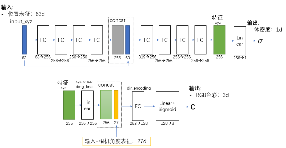
NeRF 网络
NeRF 网络默认是一个多层的MLP。中间第四层有skip connection,构成了一个ResNet的结构。网络的宽度默认为256。
输入:
-
- 位置坐标的表征(in_channels_xyz):63d
-
- 相机角度的表征(in_channels_dir):27d
输出:
-
- 体密度 \sigma:1d
-
- RGB色彩值 \mathbf{C}: 3d
网络结构:
FC指的是带ReLU的全连接层。Linear层指的是单纯的线性方程。
代码实现
class NeRF(nn.Module):
    def __init__(self,
                 D=8, W=256,
                 in_channels_xyz=63, in_channels_dir=27,
                 skips=[4]):
        """
        D: number of layers for density (sigma) encoder
        W: number of hidden units in each layer
        in_channels_xyz: number of input channels for xyz (3+3*10*2=63 by default)
        in_channels_dir: number of input channels for direction (3+3*4*2=27 by default)
        skips: add skip connection in the Dth layer
        """
        super(NeRF, self).__init__()
        self.D = D
        self.W = W
        self.in_channels_xyz = in_channels_xyz
        self.in_channels_dir = in_channels_dir
        self.skips = skips

        # xyz encoding layers
        for i in range(D):
            if i == 0:
                layer = nn.Linear(in_channels_xyz, W)
            elif i in skips:
                layer = nn.Linear(W+in_channels_xyz, W)
            else:
                layer = nn.Linear(W, W)
            layer = nn.Sequential(layer, nn.ReLU(True))
            setattr(self, f"xyz_encoding_{i+1}", layer)
        self.xyz_encoding_final = nn.Linear(W, W)

        # direction encoding layers
        self.dir_encoding = nn.Sequential(
                                nn.Linear(W+in_channels_dir, W//2),
                                nn.ReLU(True))

        # output layers
        self.sigma = nn.Linear(W, 1)
        self.rgb = nn.Sequential(
                        nn.Linear(W//2, 3),
                        nn.Sigmoid())

    def forward(self, x, sigma_only=False):
        """
        Encodes input (xyz+dir) to rgb+sigma (not ready to render yet).
        For rendering this ray, please see rendering.py

        Inputs:
            x: (B, self.in_channels_xyz(+self.in_channels_dir))
               the embedded vector of position and direction
            sigma_only: whether to infer sigma only. If True,
                        x is of shape (B, self.in_channels_xyz)

        Outputs:
            if sigma_ony:
                sigma: (B, 1) sigma
            else:
                out: (B, 4), rgb and sigma
        """
        if not sigma_only:
            input_xyz, input_dir = \
                torch.split(x, [self.in_channels_xyz, self.in_channels_dir], dim=-1)
        else:
            input_xyz = x

        xyz_ = input_xyz
        for i in range(self.D):
            if i in self.skips:
                xyz_ = torch.cat([input_xyz, xyz_], -1)
            xyz_ = getattr(self, f"xyz_encoding_{i+1}")(xyz_)

        sigma = self.sigma(xyz_)
        if sigma_only:
            return sigma

        xyz_encoding_final = self.xyz_encoding_final(xyz_)

        dir_encoding_input = torch.cat([xyz_encoding_final, input_dir], -1)
        dir_encoding = self.dir_encoding(dir_encoding_input)
        rgb = self.rgb(dir_encoding)

        out = torch.cat([rgb, sigma], -1)

        return out
体素渲染
假设我们已经得到了一束光线上所有的位置对应的色彩和体密度。我们需要对这束光线进行后处理(体素渲染),得到最终在图片上的像素值。
# z_vals: (N_rays, N_samples_) depths of the sampled positions
# noise_std: factor to perturb the model's prediction of sigma(提升模型鲁棒性??)

# Convert these values using volume rendering (Section 4)
deltas = z_vals[:, 1:] - z_vals[:, :-1] # (N_rays, N_samples_-1)
delta_inf = 1e10 * torch.ones_like(deltas[:, :1]) # (N_rays, 1) the last delta is infinity
deltas = torch.cat([deltas, delta_inf], -1)  # (N_rays, N_samples_)

# Multiply each distance by the norm of its corresponding direction ray
# to convert to real world distance (accounts for non-unit directions).
deltas = deltas * torch.norm(dir_.unsqueeze(1), dim=-1)

noise = torch.randn(sigmas.shape, device=sigmas.device) * noise_std

# compute alpha by the formula (3)
alphas = 1-torch.exp(-deltas*torch.relu(sigmas+noise)) # (N_rays, N_samples_)
alphas_shifted = \
    torch.cat([torch.ones_like(alphas[:, :1]), 1-alphas+1e-10], -1) # [1, a1, a2, ...]
weights = \
    alphas * torch.cumprod(alphas_shifted, -1)[:, :-1] # (N_rays, N_samples_)
weights_sum = weights.sum(1) # (N_rays), the accumulated opacity along the rays
                                # equals "1 - (1-a1)(1-a2)...(1-an)" mathematically
if weights_only:
    return weights

# compute final weighted outputs
rgb_final = torch.sum(weights.unsqueeze(-1)*rgbs, -2) # (N_rays, 3)
depth_final = torch.sum(weights*z_vals, -1) # (N_rays)
第二轮渲染
对于渲染的结果,会根据 对应的权重,使用pdf抽样,得到新的渲染点。例如默认第一轮粗渲染每束光线是64个样本点,第二轮再增加128个抽样点。
然后使用finemodel 进行预测,后对所有的样本点(64+128)进行体素渲染。
def sample_pdf(bins, weights, N_importance, det=False, eps=1e-5):
    """
    Sample @N_importance samples from @bins with distribution defined by @weights.

    Inputs:
        bins: (N_rays, N_samples_+1) where N_samples_ is "the number of coarse samples per ray - 2"
        weights: (N_rays, N_samples_)
        N_importance: the number of samples to draw from the distribution
        det: deterministic or not
        eps: a small number to prevent division by zero

    Outputs:
        samples: the sampled samples
    """
    N_rays, N_samples_ = weights.shape
    weights = weights + eps # prevent division by zero (don't do inplace op!)
    pdf = weights / torch.sum(weights, -1, keepdim=True) # (N_rays, N_samples_)
    cdf = torch.cumsum(pdf, -1) # (N_rays, N_samples), cumulative distribution function
    cdf = torch.cat([torch.zeros_like(cdf[: ,:1]), cdf], -1)  # (N_rays, N_samples_+1)
                                                               # padded to 0~1 inclusive

    if det:
        u = torch.linspace(0, 1, N_importance, device=bins.device)
        u = u.expand(N_rays, N_importance)
    else:
        u = torch.rand(N_rays, N_importance, device=bins.device)
    u = u.contiguous()

    inds = searchsorted(cdf, u, side='right')
    below = torch.clamp_min(inds-1, 0)
    above = torch.clamp_max(inds, N_samples_)

    inds_sampled = torch.stack([below, above], -1).view(N_rays, 2*N_importance)
    cdf_g = torch.gather(cdf, 1, inds_sampled).view(N_rays, N_importance, 2)
    bins_g = torch.gather(bins, 1, inds_sampled).view(N_rays, N_importance, 2)

    denom = cdf_g[...,1]-cdf_g[...,0]
    denom[denom<eps] = 1 # denom equals 0 means a bin has weight 0, in which case it will not be sampled
                         # anyway, therefore any value for it is fine (set to 1 here)

    samples = bins_g[...,0] + (u-cdf_g[...,0])/denom * (bins_g[...,1]-bins_g[...,0])
    return samples
Loss
这里直接使用的 MSE loss,对输出的像素值和 ground truth 计算 L2-norm loss.
训练数据
训练数据
根据前面的介绍,NeRF实现的,是从 【位置坐标 katex[/katex] 和 拍摄角度(\theta, \phi)】 到 【体密度 (\sigma) 和 RGB色彩值 (\mathbf{C})】的映射。根据体素渲染理论,图片中的每一个像素,实质上都是从相机发射出的一条光线渲染得到的。 因此,我们首先,需要得到每一个像素对应的光线(ray),然后,计算光线上每一个点的【体密度 (\sigma) 和 RGB色彩值 (\mathbf{C})】,最后再渲染得到对应的像素值。
对于训练数据,我们需要拍摄一系列的图片(如100张)图片和他们的拍摄相机角度、内参、场景边界(可以使用COLMAP获得)。我们需要准备每一个像素对应的光线(ray)信息,这样可以组成成对的训练数据【光线信息 <==> 像素值】。
下面以 LLFFDataset ("datasets/llff.py") 为例,进行分析:
读取的数据(以一张图片为例):
- 图片:尺寸是 N_{img}\times C\times H\times W。 其中 C=3 代表了这是RGB三通道图片
- 拍摄角度信息(从COLMAP生成):N_{img}\times 17。前15维可以变形为 3\times 5,代表了相机的pose,后2维是最近和最远的深度。解释: 3×5 pose matrices and 2 depth bounds for each image. Each pose has [R T] as the left 3×4 matrix and [H W F] as the right 3×1 matrix. R matrix is in the form [down right back] instead of [right up back] . (https://github.com/bmild/nerf/issues/34)
拍摄角度预处理
第一步:根据拍摄的尺寸和处理尺寸的关系,缩放相机的焦距。例如:H_{img}=3024, W_{img}=4032, F_{img}=3260, 如果我们想处理的尺寸是 H=378, W=504 (为了提升训练的速度),我们需要缩放焦距F:
F=F_{img}\times \frac{W}{W_{img}}=3260\times \frac{504}{4032}= 407# "datasets/llff.py", line:188
# Step 1: rescale focal length according to training resolution
H, W, self.focal = poses[0, :, -1] # original intrinsics, same for all images
assert H*self.img_wh[0] == W*self.img_wh[1], \
f'You must set @img_wh to have the same aspect ratio as ({W}, {H}) !'
self.focal *= self.img_wh[0]/W第二步:调整pose的方向。在"poses_bounds.npy"中,pose的方向是“下右后”,我们调整到“右上后”。同时使用 “center_poses(poses)” 函数,对整个dataset的坐标轴进行标准化(??)。
解释:“poses_avg computes a "central" pose for the dataset, based on using the mean translation, the mean z axis, and adopting the mean y axis as an "up" direction (so that Up x Z = X and then Z x X = Y). recenter_poses very simply applies the inverse of this average pose to the dataset (a rigid rotation/translation) so that the identity extrinsic matrix is looking at the scene, which is nice because normalizes the orientation of the scene for later rendering from the learned NeRF. This is also important for using NDC(Normalized device coordinates) coordinates, since we assume the scene is centered there too.”(https://github.com/bmild/nerf/issues/34)
# "datasets/llff.py", line:195
    # Step 2: correct poses
    # Original poses has rotation in form "down right back", change to "right up back"
    # See https://github.com/bmild/nerf/issues/34
    poses = np.concatenate([poses[..., 1:2], -poses[..., :1], poses[..., 2:4]], -1)
            # (N_images, 3, 4) exclude H, W, focal
    self.poses, self.pose_avg = center_poses(poses)
第三步:令最近的距离约为1。 解释:“The NDC code takes in a "near" bound and assumes the far bound is infinity (this doesn’t matter too much since NDC space samples in 1/depth so moving from "far" to infinity is only slightly less sample-efficient). You can see here that the "near" bound is hardcoded to 1”。For more details on how to use NDC space see https://github.com/bmild/nerf/files/4451808/ndc_derivation.pdf
# "datasets/llff.py", line:205
    # Step 3: correct scale so that the nearest depth is at a little more than 1.0
    # See https://github.com/bmild/nerf/issues/34
    near_original = self.bounds.min()
    scale_factor = near_original*0.75 # 0.75 is the default parameter
                                        # the nearest depth is at 1/0.75=1.33
    self.bounds /= scale_factor
    self.poses[..., 3] /= scale_factor
计算光线角度
接下来就是对每一个像素,使用“get_ray_directions()”函数计算所对应的光线。这里只需要使用图像的长宽和焦距即可计算。
self.directions = get_ray_directions(self.img_wh[1], self.img_wh[0], self.focal) # (H, W, 3)调用函数:
def get_ray_directions(H, W, focal):
    """
    Get ray directions for all pixels in camera coordinate.
    Reference: https://www.scratchapixel.com/lessons/3d-basic-rendering/
               ray-tracing-generating-camera-rays/standard-coordinate-systems

    Inputs:
        H, W, focal: image height, width and focal length

    Outputs:
        directions: (H, W, 3), the direction of the rays in camera coordinate
    """
    grid = create_meshgrid(H, W, normalized_coordinates=False)[0]
    i, j = grid.unbind(-1)
    # the direction here is without +0.5 pixel centering as calibration is not so accurate
    # see https://github.com/bmild/nerf/issues/24
    directions = \
        torch.stack([(i-W/2)/focal, -(j-H/2)/focal, -torch.ones_like(i)], -1) # (H, W, 3)

    return directions
世界坐标系下的光线
在拿到每一个像素对应的光线角度后,我们需要得到具体的光线信息。首先,先计算在世界坐标系下的光线信息。主要是一个归一化的操作。
Get ray origin and normalized directions in world coordinate for all pixels in one image. Reference: https://www.scratchapixel.com/lessons/3d-basic-rendering/ray-tracing-generating-camera-rays/standard-coordinate-systems
输入:
- 图像上每一点所对应的光线角度:(H, W, 3) precomputed ray directions in camera coordinate。
- 相机映射矩阵c2w:(3, 4) transformation matrix from camera coordinate to world coordinate
输出:
- 光线原点在世界坐标系中的坐标:(H*W, 3), the origin of the rays in world coordinate
- 在世界坐标系中,归一化的光线角度:(H*W, 3), the normalized direction of the rays in world coordinate
def get_rays(directions, c2w):
    """
    Get ray origin and normalized directions in world coordinate for all pixels in one image.
    Reference: https://www.scratchapixel.com/lessons/3d-basic-rendering/
               ray-tracing-generating-camera-rays/standard-coordinate-systems

    Inputs:
        directions: (H, W, 3) precomputed ray directions in camera coordinate
        c2w: (3, 4) transformation matrix from camera coordinate to world coordinate

    Outputs:
        rays_o: (H*W, 3), the origin of the rays in world coordinate
        rays_d: (H*W, 3), the normalized direction of the rays in world coordinate
    """
    # Rotate ray directions from camera coordinate to the world coordinate
    rays_d = directions @ c2w[:, :3].T # (H, W, 3)
    rays_d = rays_d / torch.norm(rays_d, dim=-1, keepdim=True)
    # The origin of all rays is the camera origin in world coordinate
    rays_o = c2w[:, 3].expand(rays_d.shape) # (H, W, 3)

    rays_d = rays_d.view(-1, 3)
    rays_o = rays_o.view(-1, 3)

    return rays_o, rays_d
NDC下的光线
NDC(Normalized device coordinates) 归一化的设备坐标系。
首先对光线的边界进行限定:
near, far = 0, 1然后对坐标进行平移和映射。
def get_ndc_rays(H, W, focal, near, rays_o, rays_d):
    """
    Transform rays from world coordinate to NDC.
    NDC: Space such that the canvas is a cube with sides [-1, 1] in each axis.
    For detailed derivation, please see:
    http://www.songho.ca/opengl/gl_projectionmatrix.html
    https://github.com/bmild/nerf/files/4451808/ndc_derivation.pdf

    In practice, use NDC "if and only if" the scene is unbounded (has a large depth).
    See https://github.com/bmild/nerf/issues/18

    Inputs:
        H, W, focal: image height, width and focal length
        near: (N_rays) or float, the depths of the near plane
        rays_o: (N_rays, 3), the origin of the rays in world coordinate
        rays_d: (N_rays, 3), the direction of the rays in world coordinate

    Outputs:
        rays_o: (N_rays, 3), the origin of the rays in NDC
        rays_d: (N_rays, 3), the direction of the rays in NDC
    """
    # Shift ray origins to near plane
    t = -(near + rays_o[...,2]) / rays_d[...,2]
    rays_o = rays_o + t[...,None] * rays_d

    # Store some intermediate homogeneous results
    ox_oz = rays_o[...,0] / rays_o[...,2]
    oy_oz = rays_o[...,1] / rays_o[...,2]

    # Projection
    o0 = -1./(W/(2.*focal)) * ox_oz
    o1 = -1./(H/(2.*focal)) * oy_oz
    o2 = 1. + 2. * near / rays_o[...,2]

    d0 = -1./(W/(2.*focal)) * (rays_d[...,0]/rays_d[...,2] - ox_oz)
    d1 = -1./(H/(2.*focal)) * (rays_d[...,1]/rays_d[...,2] - oy_oz)
    d2 = 1 - o2

    rays_o = torch.stack([o0, o1, o2], -1) # (B, 3)
    rays_d = torch.stack([d0, d1, d2], -1) # (B, 3)

    return rays_o, rays_d
训练数据的生成
输出分为两部分:光线的信息,和对应的图片像素值
- 对于每一束光线,按照 【光线原点(3d), 光线角度(3d), 最近的边界(1d), 最远的边界(1d)】= 8d 的格式存储。
- 光线对应的像素,RGB=3d 的格式存储。
self.all_rays += [torch.cat([rays_o, rays_d,
                                             near*torch.ones_like(rays_o[:, :1]),
                                             far*torch.ones_like(rays_o[:, :1])],
                                             1)] # (h*w, 8)
good
great